Lab 3: Filters

Indy Hendrickx21/08/2026About 7 min

Lab 3: Filters

⬇ Download as Word Open in Word, fill in your answers and photos, then save as PDF.

1. Assignment description

This lab is deliberately shorter than the others. There are no new instruments: you already know the function generator and the oscilloscope from lab 2, and you use them here exactly the same way. What is new is that you sweep the frequency and watch what a filter does with it.

You build the three filters from the theory lesson, you measure their cut-off frequency instead of only calculating it, and you change the parts to see the cut-off move.

What we expect:

Every measurement table filled in, with units
Every cut-off frequency calculated first, then measured
One graph of your own measurements
A short reflection of approximately half a page in Chapter 3

Planning

When	Steps	Time
First part of the lesson	Theory	about 1,5 h
Second part of the lesson	2.1 Low pass, find the cut-off	20 min
	2.2 The response curve	25 min
	2.3 Change R and change C	15 min
	2.4 High pass	12 min
	2.5 Band pass	18 min
If you finish early	2.6 and 2.7	not graded

What do we need?

From your own kit:

1x breadboard and jumper wires
Resistors: 1 kΩ, 10 kΩ

From the lab room:

1x function generator with a BNC test lead, 1x oscilloscope with two ×10 probes
Capacitors: 2x 1 µF, 1x 100 nF, 1x 10 nF, all non-polarized (film or ceramic)

Why not the capacitor from your kit?

The 1 µF in your kit is a tantalum type and it has a polarity, like the electrolytic capacitor from lab 2. A filter carries a signal that swings positive and negative, so a polarized capacitor is the wrong component for the job. Use the non-polarized ones from the lab room.

Two reminders from lab 2

Both scope ground clips go to the generator ground. In this lab that is easy, because the generator, the filter and the scope all share the same ground rail. There is no floating output here.
Set both probes and both channel menus to 10X, otherwise every voltage you read is ten times too small.

2. Lab

2.1 Low pass filter: find the cut-off frequency

Low pass filter with the generator and both probes

Step 1: Calculate first

You are going to build the filter with R = 1 kΩ and C = 1 µF. Calculate its cut-off frequency before you touch anything.

f_c = \frac{1}{2 \pi R C}

Step 2: Build and set up

Build the filter on the breadboard: generator to the input, resistor, then the capacitor from the output node down to the ground rail.
Generator: sine, amplitude about 6 Vpp, frequency 20 Hz to start.
CH1 probe on the input, CH2 probe on the output, both ground clips on the ground rail.
Press MEASURE and set up two measurements: Pk-Pk of CH1 and Pk-Pk of CH2.

Step 3: Look before you measure

Set these three frequencies and describe in a few words what CH2 does compared to CH1.

Frequency	What the output looks like next to the input
20 Hz
your calculated f_c
2 kHz

Step 4: Hunt for the cut-off frequency

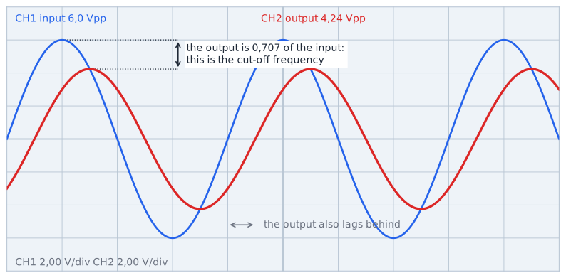
Now find the cut-off frequency by measuring instead of calculating. Turn the frequency dial slowly until CH2 is 0,707 times CH1. With 6,0 Vpp going in, that means about 4,24 Vpp coming out.

What the screen looks like at the cut-off frequency

Quantity	Value
U in (CH1 Pk-Pk)
U out at the cut-off point (0,707 × U in)
Frequency where you found it
Your calculated f_c from step 1
Difference in percent

Take a picture of the screen at the cut-off frequency, with both traces visible.

Besides being smaller, the output does something else at this frequency. What do you see?

2.2 The response curve

One point is a measurement. A curve is a filter.

Step 1: Sweep

Keep the same circuit. Set each frequency below, read both Pk-Pk values, and calculate the ratio. Record CH1 every time as well, because the generator does not keep exactly the same amplitude at every frequency.

The output gets small

Above the cut-off frequency the output shrinks fast. Turn the CH2 VOLTS/DIV knob to a smaller setting so the trace stays readable. That does not change the measurement, only the zoom.

Frequency	U in (Vpp)	U out (Vpp)	U out / U in
20 Hz
50 Hz
100 Hz
160 Hz
300 Hz
1 kHz
3 kHz
10 kHz

Step 2: Draw the curve

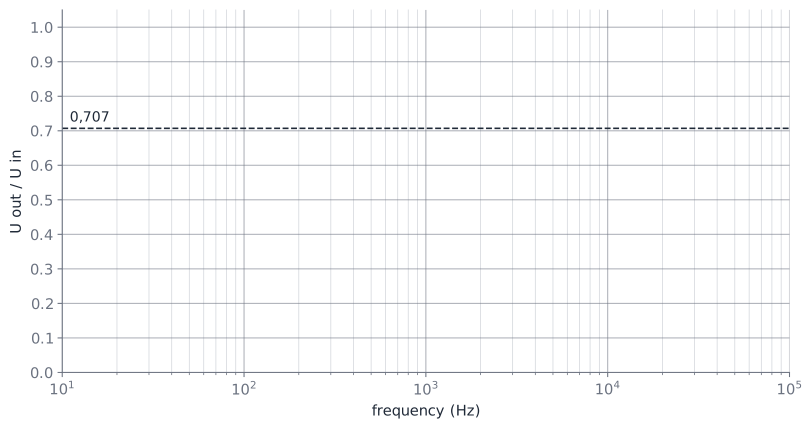
Plot your ratios on the grid below. The horizontal axis is logarithmic, which is why the frequencies you measured are spread out evenly across it.

Empty graph paper with a logarithmic frequency axis

Step 3: Two checks

The theory gives you two things to check without any extra formula.

Check	What the theory says	What you measured
The ratio at 160 Hz	about 0,707
The ratio at 1,6 kHz, one decade higher	about 0,1

Does your curve have the same shape as the graph in the theory lesson? Name one thing that is different, and say why you think that is.

💡 Think about the tolerance of your parts and about how accurately you can read a small trace.

2.3 Change R, change C

The formula says the cut-off frequency depends on R and C together. Time to prove it.

Step 1: Ten times the resistor

Replace the 1 kΩ with 10 kΩ and keep the 1 µF.

Calculate the new cut-off frequency first.
Then find it on the scope with the 0,707 method.

Step 2: A tenth of the capacitor

Put the 1 kΩ back and replace the capacitor with 100 nF.

Calculate first.
Then measure.

R	C	f_c calculated	f_c measured
1 kΩ	1 µF
10 kΩ	1 µF
1 kΩ	100 nF

One of these changes made the cut-off frequency ten times lower and the other made it ten times higher. Which did what?

Without building it: what cut-off frequency would you get with 10 kΩ and 100 nF? Compare your answer with the first row of the table and explain what that tells you.

💡 Look at what R and C do inside the formula.

2.4 High pass filter

Same two parts, swapped.

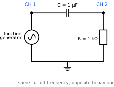
High pass filter with the generator and both probes

Rebuild with R = 1 kΩ and C = 1 µF, but now the capacitor is in the signal path and the resistor goes from the output node to ground.

Frequency	U in (Vpp)	U out (Vpp)	U out / U in
20 Hz
50 Hz
160 Hz
500 Hz
3 kHz

Quantity	Value
f_c calculated
f_c measured with the 0,707 method

You used exactly the same resistor and the same capacitor as in step 2.1. Compare the two cut-off frequencies, and compare the two behaviours.

2.5 Band pass filter

Put the two together and only a band of frequencies survives.

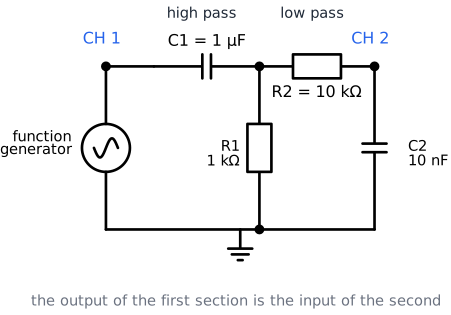
Band pass filter: a high pass section followed by a low pass section

Build: high pass section with C1 = 1 µF and R1 = 1 kΩ, then a low pass section with R2 = 10 kΩ and C2 = 10 nF. CH1 stays on the input, CH2 moves to the output of the second section.

Step 1: Calculate both cut-off frequencies

Step 2: Measure across the whole range

Frequency	U in (Vpp)	U out (Vpp)	U out / U in
20 Hz
100 Hz
160 Hz
500 Hz
1,6 kHz
5 kHz
20 kHz

Step 3: Find the band

Sweep the frequency slowly and look for the point where the output is at its largest. Then find the two frequencies where the output has dropped to 0,707 of that maximum.

Quantity	Value
Largest output you can reach, and at which frequency
Lower cut-off frequency (0,707 of the maximum)
Upper cut-off frequency (0,707 of the maximum)
Bandwidth (upper minus lower)

Take a picture of the screen in the middle of the pass band, and one well outside it.

In the middle of the band the output is still smaller than the input, even though both sections should be passing the signal. Where does the missing voltage go?

💡 The second section is connected across the first one. Reread the last paragraph of the higher orders section in the theory.

2.6 Extra: a square wave through the filter

Steps 2.6 and 2.7 are optional and are not graded.

Rebuild the low pass filter with 1 kΩ and 1 µF, and switch the generator from sine to square at 20 Hz.

Frequency	What the output looks like
20 Hz
160 Hz
1 kHz

The sharp corners of the square wave become rounded. Which curve from lesson 2 does the output remind you of, and why does that make sense?

💡 A square wave is a supply that is switched on and off. What was the capacitor doing in that circuit?

2.7 Extra: design one yourself

Using only the parts on your table, design a low pass filter with a cut-off frequency as close as possible to 500 Hz.

Choose R and C and calculate what cut-off you will get.
Build it and measure the real cut-off frequency.
Note how far off you are, and whether a different pair would have been closer.

3. Reflection

Write a short reflection of approximately half a page (font: Arial 9.5). Answer the following questions in your own words.

What did you learn?

Which concepts from the theory lesson did you recognise in the lab? Give a concrete example from your own measurements.

What was difficult?

Which step gave you the most trouble? How did you solve it?

Calculated against measured

Your measured cut-off frequencies were never exactly equal to the calculated ones. Name two causes, and say which one you think mattered most.

Connection to IoT

You connect an analogue sensor to a microcontroller and the readings jump around because of electrical noise. Which of the three filters from this lab would you put between the sensor and the input pin, and how would you choose R and C for it?